Your cookie choices
Essential cookies keep your basket and sign-in working. Optional cookies help us understand visits and measure ads. Privacy details.
Essential cookies keep your basket and sign-in working. Optional cookies help us understand visits and measure ads. Privacy details.
How neural networks learn by following the slope
AI-assisted explanation. It may contain errors; use a textbook or original source to check important details.
Imagine you’re hiking in thick fog on a landscape of hills and valleys, and your goal is to find the lowest point. You can’t see the whole terrain, but you can feel the slope right where you stand. Gradient descent is the rule that says: “Take a small step downhill from where you are right now.” In the equation θ := θ − α ∇θ J(θ) you can think of it as a repeated recipe for improving a model: - θ (theta) is the collection of “knobs” your model can turn—its parameters (like weights in a neural network). - J(θ) is a score that tells you how bad your model currently is (often called the loss or cost). Lower is better. - ∇θ J(θ) (the gradient) is the “slope arrow” of the loss with respect to the parameters: it points in the direction where J increases fastest. It’s like a compass that points uphill. - The minus sign means we go the opposite way—downhill, toward smaller loss. - α (alpha) is the learning rate, the step size. Too big and you can overshoot or bounce around; too small and learning becomes painfully slow. - := means “update/replace”: after computing the right-hand side, we overwrite θ with the new value. So the story of the equation is: compute which way makes the error worse (the gradient), then nudge the parameters a little in the opposite direction so the error gets smaller. Repeating this many times is how a model “learns” from data.
Gradient descent comes from a much older mathematical dream: optimizing something by following its slope. Long before machine learning, scientists and engineers wanted systematic ways to minimize error—whether in fitting astronomical observations, designing structures, or tuning control systems. A key ancestor is least squares (early 1800s), where researchers needed to fit models to noisy data. Once people began expressing “fit” as an explicit function to minimize, it became natural to ask: how do you actually find the minimum? The modern iterative idea—start somewhere and repeatedly step in a direction that reduces the objective—was formalized in the 20th century. A landmark moment is Cauchy’s method of steepest descent (1847), which framed minimization as repeatedly moving opposite the gradient. Later, as computing developed, these iterative methods became practical and central. In machine learning, gradient descent became the workhorse because many models are too large and complex for closed-form solutions; yet their gradients can often be computed efficiently (especially after backpropagation made gradients in neural networks practical).
Pioneered by: The core idea is commonly credited to Augustin-Louis Cauchy, who introduced the method of steepest descent in 1847. The exact update form used in machine learning is a standard expression of that idea applied to parameter vectors θ and a loss function J(θ).